SedSimple auxiliary programs

Copyright (c) 2025 Westchase Software Corporation

Rev 1.15 July 2025

INTRODUCTION

This document describes a set of computer programs that work in conjunction with SedSimple. While none of these programs is required for producing a SedSimple model, they help to format input and post-process output. All of these programs work from the command line. Normally, this entails opening a command window (or a “terminal” in Linux or Mac). Then to run them, enter the name of the program and the corresponding files or parameters (as described in this documentation).

A summary of these programs follows (click on the underlined paragraph headers to go directly to the detailed documentation of each program):

Reformatting

ToKVL: Converts several common formats for surfaces used in industry (IRAP, EarthVision Grid, and ZMAP) to the kvl format used by SedSimple. This program is commonly used while preparing data for SedSimple.

GConv: Converts a SedSimple result model to an hdf5 file readable by external industry programs. Sirius will also be able to read the hdf5 format. Although hdf5 is known to be “fast”, the particular subset of hdf5 generated by this program is adapted to specific external programs and is relatively slow.

ToXYZ: Converts a SedSimple result model to points as X-Y-Z-value data, or to Earth Vision format.

Regularize: Regularizes a SedSimple result model, i.e. it converts the model to a regular 3D Cartesian grid of equal “shoebox” cells. This may be useful for geostatistical or flow-modeling programs that require regular regular grids.

Data extraction

SedWells: Extracts synthetic vertical wells from a SedSimple result model, or from a model post processed by one of the programs described above (for example a model containing porosity and permeability estimates.

SedXtract: Extracts a subset of a SedSimple result model. The subset is defined by the limits of a Cartesian box. This may be useful for trimming the edges of a model or for displaying only the significant part of a model in order to gain display speed.

Post processing

SedTop: Places a SedSimple result model in depth to match seismic and logs and optionally adds an overburden. It also provides a measure of error between the SedSimple thickness and the thickness seen in seismic or well logs.

SedPost: Post processes a SedSimple result model to produce: layer thicknesses, depth of deposition, overburden, porosity, horizontal permeablity, and vertical permeability.

Statistics

SedVAvg: Produces vertical averages (within any interval of contiguous layers) of any properties in a SedSimple result model.

SedStats: Produces statistics from multiple SedSimple result models. All models must have the same dimensions (number of cells and properties). This is useful for Monte Carlo methods, in which the user may vary one or more input parameters randomly or systematically and obtain statistics of resulting properies.

WORKFLOW

The exact way in which these programs are used in conjunction with SedSimple depends on the data available and the objectives of the study. As a general outline, the following graph shows how these programs may be used in a workflow.

INSTALLATION AND USAGE

To install the auxiliary programs, simply unzip the file sedaux.zip, which contains all executables and this documentation in pdf format. Place the executables in a directory that is in your PATH (consult your operating system documentation to find how to set the PATH environment variable). Typically, this directory would be the same as the one where the sedsimple executable is located.

To run a program type its name at the command prompt followed by any parameters as described in this documentation. If all parameterd are omitted, the program will provide a brief help message describing the required parameters.

DETAILED DESCRIPTIONS

ToKvl

ToKvl converts common 2D formats (IRAP, EarthVision Grid, and ZMAP) to .kvl (the format used by SedSimple).

Usage

This program is typically used to produce a kvl file to be used as initial topographic surface for SedSimple, from a file produced by a commercial program (for example a program that digitizes seismic reflectors). It can also be used to convert other properties, such as sediment proportions, to be used as “basement” compositions for SedSimple.

To run the program, enter the following command:

> tokvl filein.[ext] fileout.kvl

where:

• filein.[ext] is the input file. [ext] represents an extension that must be one of the following:

  • irp or irap for IRAP format files
  • evg or evis for Earth Vision Grid format files
  • zmp or zmap for ZMap format files

• fileout.kvl represents the name of the output file. Its extension must always be kvl. If the output file exists, it will be overwritten.

It is usually necessary to edit the resulting kvl file to provide the correct name for the variable needed. For example, if the property converted represents a surface to be used as basement top in a SedSimple input file the name of the property should be TOP (please refer to the SedSimple documentation for details)).

Algorithm

The algorithm works only on 2D regular grids (representing surfaces). It simply reads all values and converts them to a valid kvl file.

GConv

GConv (short for “Geo Convert”) converts files used in geologic process modeling. The present version of GConv can only convert from SedSimple kvl output files to hdf5 files that can be imported into applications provided by other vendors. The output hdf5 files can also be viewed by the program Sirius, although Sirius can display kvl output files directly, without the need for conversion.

Usage

To run GConv, enter the following command:

> gconv infile.kvl outfile.hdf5

where:

• infile.kvl is an input kvl file (that results from the output of the program SedSimple)
• outfile.hdf5 is the desired output file. The latter can then be imported into an application that requires this type of file.

Remarks

The hdf5 file resulting from the conversion is meant for display by other programs that may have better capabilities for further processing and integration with other data. Files in hdf5 format can also be opened by the Sirius graphics program. However, this format also has the following drawbacks:

1. Although the hdf5 file format is widely used for scientific data and is inherently fast, its usage for geologic data applies a specific and quite complex structure to the data. This can make conversions to hdf5 as well as reading hdf5 files slower than the native kvl format.
2. The external programs that can read hdf5 files cannot show some of the details shown by the Sirius program. Conversion to hdf5 with GConv downgrades the information to make it displayable by other programs. These issues may be minor but can be visible. They include:
   1. Display of tie-centered data in cross sections and node-centered data in plan
   2. Diagonal-smearing artifacts
   3. Display of local erosional features For more information on these issues, please refer to the following paper:

For these reasons, it is recommended to use the native kvl format and the program Sirius for display to avoid these issues, unless it is important to integrate the information with other data in ways that are not available in Sirius.

Algorithm

The algorithm is not described in detail here. The conversion is not a straight conversion to hdf5. The program reorganizes the properties to make them readable by external programs such as Petrel-GPM¹. Among other things, the conversion involves adding a time dimension to the data. Adding the time dimension is a lengthy process. It may take several minutes to process a file. The time is generally proportional to the number of time steps. Despite being a binary file, the result file may be many times larger than the original kvl file. The generated file can be read by Sirius, but it will be slower to read than the kvl file. Note that the Sirius program is capable of reading the output file of Petrel-GPM directly, with no intervening conversion. Thus, the program GCconv provides a two-way connection between SedSimple and Petrel-GPM. Output of SedSimple can be read into Petrel-GPM and then converted to Petrel grids and exported to any other format supported by Petrel.

ToXYZ

ToXYZ processes the output of SedSimple or any set of 2D properties (surfaces) contained in a kvl file and rewrites them in the form of X-Y-value points and 3D grids as X-Y-Z-value ASCII files. This is useful for exporting the results to other formats based on X, Y, Z, points. It can also write Earth Vision Grid format files.

Usage

To run the program, enter the following command:

> toxyz sedsimple_out.kvl parmfile.kvl result.[xyz][evg]

where:

• sedsimple_out.kvl is the name of a SedSimple output file (which is the input to this program)
• parmfile.kvl is the name of a file containing parameters that are necessary for processing. The format and content of this file are described below
• result.[xyz][evg] is the name of the output file of ToXYZ. If the extension is xyz, the result will will be in the form of X, Y, Z, value points. If the extension is evg the result will be in Eath Vision Grid format.

Parameter file

The file parmfile.kvl is a kvl file that must contain single-value parameters. All parameters are optional. The possible parameters are:

• XCELLSIDE: Size of the x-axis side of a cell as used in SedSimple, typically in meters (but it could be in another unit (e.g. feet) if the X, Y, Z, results are desired in that unit. Default: 1.0
• YCELLSIDE: Size of the y-axis side of a cell. typically the same as XCELLSIDE because cells are square in SedSimple. Default: 1.0
• XORIGIN: X coordinate of the origin of the SedSimple grid (node 0,0) in the desired coordinate system. Default: 0.0
• YORIGIN: Y coordinate of the origin of the SedSimple grid (node 0,0) in the desired coordinate system. Default: 0.0
• ROTATION: Rotation in degrees from North of the SedSimple grid relative to the desired coordinate system. Default: 0.0

If any parameter is missing, the algorithm will use the default value noted above. If using all default values, the coordinates will be in units of grid cells.

The following illustration should help to clarify the meaning and usage of these parameters.

Example parameter file

An example of a parameter file follows. It assumes the same parameters as in the preceding figure:

XCELLSIDE = 75
YCELLSIDE = 75
XORIGIN = 350
YORIGIN = 250
ROTATION = 30

Algorithm

The algorithm converts the coordinates of every node into the external coordinate system according to the parameters provided. Then it writes each coordinte followed by the property values.

Regularize

“Regularize” the output of SedSimple (consisting of a kvl format file) to an ASCII file containing a 3D array of values representing a regular rectangular grid of cells corresponding to one of the properties (user selected) in the kvl file. It admits a number of parameters to control the resolution of the output.

This program is useful because SedSimple (as well as many other stratigraphic and geocellular modeling programs) writes the output to cells that are not regular. Furthermore, cells may be partly or fully truncated by erosion. However, geostatistical and image analysis programs usually require a “rasterized” or regular grid consisting of equal rectangular boxes.

Usage

To run the program, enter the following command:

> regularize sedsimple_out.kvl result.txt [parmfile.txt]

where:

• sedsimple_out.kvl is the name of a SedSimple output file (which is the input to this program)
• result.txt is the name of the output file of Regularize
• [parmfile.txt] is an optional parameter file containing numbers and strings. If the file is not given, the program will ask for the needed information interactively.

The format of the output file consists of several layers separated from one another by a blank line. Each layer consists of a rectangular array of rows and columns of numbers. The layers are ordered from bottom to top (the first layer in the file is the stratigraphically lowest). The lines in each layer are ordered from South to North (the first line in the layer is to the South). The numbers within the line are ordered from West to East (the leftmost number is to the West).

Parameter file

The parameter file is not a kvl format file. It is an ASCII file containing the value of parameters that are otherwise asked interactively. The best way to prepare this file is to run the program interactively first and then prepare an ASCII file with the entries. There are only 4 entries:

1. Name of the property to be regularized. This is the “keyword” of the property in the kvl file, for example “SED1”. The property must of course exist in the kvl file. Only one property is processed at a time. In order to extract more than one property or combine the output of properties (for example, producing a facies identification number from several sediment fractions) the user must run the program repeatedly or write his/her own automatization scripts or programs.

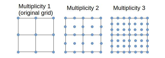
2. Horizontal multiplicity. This is an integer greater than or equal to 1 that represents the new number of nodes (on a line in the grid) for each original node. For example a grid that has 3 by 3 nodes (2 by 2 cells), will have the following number of nodes and cells for each multiplicity value:

   Multiplicity	Nodes	Cells
   1	3 * 3	2 * 2
   2	5 * 5	4 * 4
   m	((nx-1)m+1) * ((ny-1)m+1)	(nx-1)m * (ny-1)m

   nx and ny are the original numbers of nodes on each axis.

   The following figure illustrates the multiplicity concept:

   

   The program works with nodes rather than cells. However, this distinction is usually not significant for geostatistical programs, because a regular “node centered” grid can usually be considered equivalent to a “cell centered” grid displaced by half a cell in both directions. The resulting grid shows the value at a single point that coincides with the node point horizontally, and the center of the regular layer vertically. The program does not integrate over the interval represented by the regular layer, but samples a single point. Integration may be implemented in a future version.

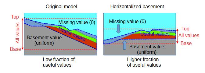
3. Whether or not to “horizontalize” the basement. This is a Boolean value represented by a letter (’Y” for “yes” and “N” for “no”) and indicates whether the basement should be horizontalized. Horizontalizing the basement will produce a grid in which the original basement surface is horizontalized or flattened. This is useful because the output of stratigraphic forward models is often very thin compared to the total range of elevations, especially when the basement is very tilted. Not using horizontalization would result in a very thin tilted layer, with the majority of values being basement or above surface. The following figure illustrates this concept. Notice that the “useful values” are not necessarily areally uniform; they may vary laterally but are shown in a uniform color for simplicity.

   

4. Vertical cell thickness. This is the thickness (in the same units as the original TOP property) of each output layer. The vertical interval is automatically set from the TOP property (after horizontalizing the basement if that option was requested). The cell thickness and vertical interval automatically determine the number of layers in the output grid.

An example of a parameter file follows:

SED1
2
Y
0.1

These values correspond to the parameters described in point 1 through 4 above.

Algorithm

The program generates a conceptual regular grid and consults the SedSimple output file to find out the value of the desired property at the center of each cell. Because SedSimple layers may be very thin, they might be missed between the centers of two superimposed or adjacent layers.

The program Regularize is meant to produce files that are readable by external programs. This often entails writing a script to convert to other fromats. However, because the output is simply a rectangular array of numbers, this task is relatively easy.

Presently, the program Sirius (used for graphic display of SedSimple results) cannot show regularized files directly. However, there are many programs that show regular 3D rectangular grids. Also, with some extra manual or programming work, it is possible to generate a file with regular parallel “layer-cake” tops and the regularized values as a property. This can be shown presently with Sirius.

SedWells

SedWells produces virtual wells from the output of SedSimple and a set of X-Y coordinates (one pair of coordinates per well). The result for each well is a file with X-Y-Z-values coordinates, where “values” represents one or more numbers for each property. For results corrected to present day, the file should have been processed by SedTop and grid coordinate information should be provided in the parameter file (see below).

Usage

To run the program, enter the following command:

> sedwells sedsimple_out.kvl parmfile.kvl result.xyz

where:

• sedsimple_out.kvl is the name of a SedSimple output file (which is the input to this program)
• parmfile.kvl is the name of a file containing parameters that are necessary for processing. The format and content of this file are described below
• result.xyz is the name of the output file of SedWells. The result will will be in the form of X, Y, Z, value points. If the extension is evg the result will be in Eath Vision Grid format.

Parameter file

The file parmfile.kvl is a kvl file that must contain single-value parameters. All parameters except XYWELLA are optional. The possible parameters are: - CELLSIDE: Size of the x- and y-axis side of a cell as used in SedSimple, typically in meters (but it could be in another unit (e.g. feet) if the X, Y, well coordinates are given in that unit. Default: 1.0 - XORIGIN: X coordinate of the origin of the SedSimple grid (node 0,0) in the desired coordinate system. Default: 0.0 - YORIGIN: Y coordinate of the origin of the SedSimple grid (node 0,0) in the desired coordinate system. Default: 0.0 - ROTATION: Rotation in degrees from North of the SedSimple grid relative to the desired coordinate system. Default: 0.0 - XYWELLS: Two columns of x and y external coordinates of vertical wells to extract.

The first four parameters specify a coordinate transformation very similar to that used by the program ToXYZ (refer to the ToXYZ documentation). The only difference is that SedWells uses a single parameter for the cell sides in both the X and Y directions.

If any parameter is missing, the algorithm will use the default value noted above (except for the XYWELLS parameter). If using all default values, the coordinates will be in units of grid cells.

Example parameter file

An example of a parameter (using external coordinate similar to those shown in the ToXYZ documentation) follows:

CELLSIDE = 75
XORIGIN = 350
YORIGIN = 250
ROTATION = 30
XYWELLS =
  610 415
  650 150
  400 250

Algorithm

The algorithm locates the exact cell position of each well and extracts the tops and properties along a vertical line (interpolating between cell corners using a bilinear interpolation function).

Then it writes the wells to the output file, separating each well with a blank line. The welll information consists of columns containing:

• X coordinate
• Y coordinate
• Z coordinate of each top
• Properties (one column per property)

The result will have the same resolution as the SedSimple model, which is usually low compared to a real well log. Nevertheless, the result can be used for comparison with well logs. SedXtract =========

SedXtract processes results from SedSimple to produce a model that includes only a selected portion of the original model. The selected portion is defined by the user as a range of nodes along the X and Y axes and optionally as a range of layer numbers. the result only shows the final (youngest) model, not the entire depositional and erosional history. This is useful to speed up display of a final model and show only the relevant portion at the end of modeling.

Usage

To run the program, enter the following command:

> sedxtract sedsimple_out.kvl result.kvl [xmin xmax ymin ymax
[zmin zmax]]

where:

• sedsimple_out.kvl is the name of a SedSimple output file (which is the input to this program)
• result.kvl is the name of the output file of SedXtract
• [xmin xmax ymin ymax] are four optional integers that denote the minimum and maximum node numbers in the X and Y directions respectively to include in the extracted portion. All must be >= 0 and xmin < xmax, and ymin < ymax. If they are omitted, the entire model will be extracted (this is not the same as the original model because only the final state is saved)
• [zmin zmax] are two optional integers that indicate the lowest and highest layer to extract. These parameters can be given only if the previous four parameters (xmin xmax ymin ymax) are also given. Both must be >= 0 and zmin < zmax

Algorithm

The program performs the following:

1. If the TECTONICS property is present, it adds the last (youngest) TECTONICS surface to all TOP entries and removes the TECTONICS property.

2. It changes the TOP to account for erosion (so no TOP is higher than a stratigraphically younger TOP).

3. It extracts the sub rectangle (if specified) of TOP and all other properties

4. It writes the results for all properties

SedTop

SedTop adjusts a sequence that results from SedSimple to match a given base, top and/or isopach. The sequence is compressed or expanded to match the given base, top and/or isopach. The program also provides an estimate of the thickness error incurred when imposing a new thickness (refer to the “Algorithm” section below for an explanation of the error).

Usage

To run the program, enter the following command:

> sedtop sedsimple_out.kvl parmfile1.kvl [parmfile2.kvl] result.kvl

where:

• sedsimple_out.kvl is the name of a SedSimple output file (which is the input to this program)
• parmfile1.kvl is the name of a file containing one or both of the surfaces needed by the program. The format and content of this file are described below.
• [parmfile2.kvl] is the name of an optional file containing parameters the second surface needed by the program. It is used only if the first file (parmfile1.kvl) contains only one of the surfaces
• result.kvl is the name of the output file of SedTop

Parameter files

The files parmfile1.kvl and optional parmfile2.kvl must jointly contain any two of the following three properties representng surfaces (rectangular arrays of elevation values), normally taken from seismic or wells:

• PRESENT_BASE: Present-day elevation of the base of the model, in meters (positive upward) relative to the same reference as the SedSimple files (normally present-day sea level)
• PRESENT_TOP: Preset-day elevation of the top of the model
• PRESENT_ISOPACH: Present-day isopach of the model

These surfaces must have the same number of nodes (in both the X and Y directions) as the SedSimple output model.

These files must be in kvl format (refer to the SedSimple documentation for more information). INCLUDE directives are not recognized in these files.

The program will still run if only one of these is provided (refer to the section on “Algorithm” below.

Overburden modeling

In addition to placing the model on depth, SedTop can also model overburden (a thick layer of undifferentiated composition on top of the new model). This is important not just for aesthetic reasons but also to correctly model porosity and permeability die to compaction (using the program SedPost, described later in this document) as well as to run external programs that produce synthetic seismic or model flow.

To model overburden, the parameter files may optionally inclorporate at most one of the following two optional parameters, whose values are single numbers:

• OVB_LEVEL: Level (in meters above model reference) to which the model resulting from this program will fill with overburden. The top of the overburden will be a horizontal surface at the given level.
• OVB_THICK: Thickness (in meters) of the overburden. The top of the overburden will be the new top of the model plus the given constant thickness.

If neither of these parameters are provided, the program will not model any overburden.

Example parameter file

An example of a parameter file follows. It assumes that the SedSimple model contains 10 x 10 nodes (9 x 9 cells):

PRESENT_BASE =
   0  -80 -162 -244 -324 -406 -488 -568 -650 -732
-140 -222 -302 -384 -466 -546 -628 -710 -790 -872
-280 -362 -444 -524 -606 -688 -768 -850 -932 -1012
-422 -502 -584 -666 -748 -828 -910 -992 -1072 -1154
-562 -644 -726 -806 -888 -970 -1050 -1132 -1214 -1294
-704 -784 -866 -948 -1028 -1110 -1192 -1272 -1354 -1436
-844 -926 -1006 -1088 -1170 -1250 -1332 -1414 -1496 -1576
-986 -1066 -1148 -1230 -1310 -1392 -1474 -1554 -1636 -1718
-1126 -1208 -1288 -1370 -1452 -1532 -1614 -1696 -1776 -1858
-1266 -1348 -1430 -1510 -1592 -1674 -1754 -1836 -1918 -2000

PRESENT_TOP =
   0  -40  -81 -122 -162 -203 -244 -284 -325 -366
 -70 -111 -151 -192 -233 -273 -314 -355 -395 -436
-140 -181 -222 -262 -303 -344 -384 -425 -466 -506
-211 -251 -292 -333 -374 -414 -455 -496 -536 -577
-281 -322 -363 -403 -444 -485 -525 -566 -607 -647
-352 -392 -433 -474 -514 -555 -596 -636 -677 -718
-422 -463 -503 -544 -585 -625 -666 -707 -748 -788
-493 -533 -574 -615 -655 -696 -737 -777 -818 -859
-563 -604 -644 -685 -726 -766 -807 -848 -888 -929
-633 -674 -715 -755 -796 -837 -877 -918 -959 -1000

OVB_THICK = 1000

This file specifies a new base and top to which the model will be fitted. An overburden of 1000 m will be added on top.

Algorithm

The algorithm shifts and deforms the resulting sequence vertically to force the new sequence to fit exactly between the new base and top surfaces given (or one of the two surfaces and an isopach).

If only one of the three possible 2D input grids are provided then the algorithm acts as follows:

If only PRESENT_BASE is provided, the base of the model will be shifted to the base provided, and the thickness will not change.

If only PRESENT_TOP is provided, the top of the model will be shifted vertically so that the top fits the surface provided and the thickness will not change.

If only PRESENT_ISOPACH is provided, the base will remain as it is and the top will be adjusted to fit the given isopach.

Overburden

The overburden consists of a single thick layer, whose composition is set arbitrarily to contain equal proportions of all the sediments present in the model. If stratigraphic detail of the overburden is desired, it must be modeled with a separate run of SedSimple.

The fact that a homogeneous overburden is generated may seem too trivial. It is of course a simplification, but it is crucial to have an overburden for the program SedPost (described later in this document) to properly (albeit approximately) calculate porosities and permeabilities.

Error estimates

At the end of the run, the program displays two types of error that describe the mismatch between the original thickness and the new thickness. If the thickness has not changed (for example, if the user provided only a new base, but no new top or isopach) then there will be no thickness error. The sequence may be deformed, but that can be assumed to be a normal consequence of post depositional vertical tectonics.

The thickness “error” is not always a mistake. Normal compaction may cause a significant reduction of thickness after deposition that is completely normal. It is up to the user to interpret the errors adequately according to the goals of the study.

Two measures of thickness error are provided:

1. Mean thickness error: Indicates in one number the relative thickness of the model with respect to the present day thickness. It can be positive or negative. If positive, the model exceeds the target; if negative, model does not reach target. In general it should be less than 10%.
2. Mean shape error: Root mean square of thickness differences relative to target thickness. It can only be positive (or 0). It measures local errors in thickness. In general, it should be less than 20%.

Normally, the user should try to optimize the parameters of the SedSimple run to ensure that both errors are as small as possible in absolute value. It is convenient to first try to bring the mean thickness error (which can be positive or negative) as close as possible to 0 by increasing or decreasing the overall sediment input, intensity of the transport processes, and possibly subsidence. Then the user should try to adjust the mean shape error (which can only be positive) to bring it as close as possible to 0 by adjusting the SedSimple parameters to ensure the local thickness of the model matches the present day isopach. This might involve adjusting local subsidence, basin lows areas of deltaic deposition, etc.

SedPost

SedPost processes the output of SedSimple to add useful geological and petrophysical information, such as layer thicknesses, depth of deposition, layer by layer local overburden thickness, porosity, horizontal permeablity, and vertical permeability. For present day results (as opposed to results at the end of the simulated geologic period) it is necessary to run the program SedTop first (refer to the documentation for SedTop, earlier in this document).

Usage

To run the program, enter the following command:

> sedpost sedsimple_out.kvl parmfile.kvl result.kvl

where:

• sedsimple_out.kvl is the name of a SedSimple output file (which is the input to this program)
• parmfile.kvl is the name of a file containing parameters that are necessary for processing. The format and content of this file are described below
• result.kvl is the name of the output file of SedPost

Parameter file

The files parmfile.kvl is a kvl file that must contain single-value parameters needed for processing. The names of these parameters carry a suffix (from 1 to the number of sediments in the SedSimple model). There must be one set of parameters for each sediment type. The parameters (for sediment type 1) are the following:

• POR1_0: SED1 porosity (fraction 0 to 1) at deposition (depth 0)
• POR1_1000: SED1 porosity (fraction 0 to 1) at 1000 m depth
• PERM1_0: SED1 horiz. permeability (mD) at deposition (depth 0)
• PERM1_1000: SED1 horiz. permeability (mD) at 1000 m depth
• PERMRATIO1: SED1 permeability ratio (hor/vert) at any depth after burial

For sediment type 2, the parameter names are the following: - POR2_0 - POR2_1000 - PERM2_0 - PERM2_1000 - PERMRATIO2

and so on for all sediment types.

The suffixes “0” and “1000” (for the first four of the parameters) indicate the depth at which the property applies. They are hard coded and cannot be changed. The user must specify the values for the sediment at those 2 different depths (0 and 1000 m). Of course it is unlikely that these values will be reliably available directly, so it is necessary to interpolate them from a compaction curve, or find similar values in the literature.

Notice that all parameters are for pure sediment types, which generally have higher porosities and permeabilities than the corresponding mixtures. For example a sand with 30% porosity mixed with a silt of 30% porosity results in a mixture of less than 30% porosity (and lower permeability than either component as well). The algorithm (refer to the description below) takes into account these effects and calculates a reasonable values for the mixtures.

Example parameter file

An example of a parameter file follows. It assumes that the SedSimple model contains three sediment types:

POR1_0 = 0.40
POR1_1000 = 0.15
PERM1_0 = 1000
PERM1_1000 = 100
PERMRATIO1 = 100
POR2_0 = 0.30
POR2_1000 = 0.10
PERM2_0 = 500
PERM2_1000 = 200
PERMRATIO2 = 50
POR3_0 = 0.18
POR3_1000 = 0.05
PERM3_0 = 200
PERM3_1000 = 32
PERMRATIO3 = 1

Algorithm

The algorithm for layer thicknesses is straightforward. It results in the final thickness (in meters) of each layer (always greater than or equal to 0). Any erosion that occurred after deposition is discounted fromk the thickness.

Depth of deposition is clculated relative to sea level at the time of deposition. It is positive downward (i.e. sea level minus sedimentary column surface) and is expressed in meters.

Overburden thickness is the thickness of sediment (in m) above each point. If the program SedTop has been run to add an overburden, it is counted in the overburden value.

Porosity and permeability

The program first calculates porosity, and then uses it (together with the provided parameters) for a regression with permeability.

The algorithm to estimate porosity of a seddiment mixture is as follows: Imagine you run the following conceptual experiment:

• Successively mix in sediment fractions from coarse to fine.
• The fractions fi add to 1 and represent the volume fraction of solids.
• Every fraction added occupies a volume equal to its grain volume plus its pore volume.
• The new fraction added first uses the “available” pore space, which is equal to the previous pore space minus the “unavailable” pore space. In turn the “unavailable” pore space is equal to the number of old particles times the pore volume of one new particle.
• In the end, the porosity of the mixture is equal to the pore volume divided by the total volume.

In more detail:

1. Take one unit volume of solid particles of a sediment mixture and separate it into fractions of decreasing grain size. Start with coarsest fraction:
   1. If Case a (added volume does not fill available space): The new pore volume is the previous pore volume minus the solid volume of the new fraction: (V2 = V1-f2)
   2. If Case b (added volume fills available space): The new pore volume is the pore volume of the new fraction: (V2 = f2 x p2 / (1-p2))
2. Add a new (finer) fraction: Go back to point 2 (subindex ‘1’ becomes ‘i’ and subindex ‘2’ becomes ‘i+1’)
3. In the end, porosity of the mixture is the solid volume (sum of solid fractions, which is 1) over (1+VN), where VN is the last pore volume. Therefore: Ptotal = 1/(1+VN)

The porosities of the components are provided as parameters at the surface (depth 0) and at 1000 m. They are interpolated (non linearly) to any depth assuming an inverse exponential decay and porosity 0 at infinite depth. Thus, the porosity of a mixture can be obtained at any depth. The depth used is the overburden value (also output by the program).

The calculation of permeability of a sediment mixture is based on a regression between porosity and permeability. This regression utilizes two porosity-permeability pairs for each sediment type, given by the user. The first pair corresponds to initial deposition (depth 0) while the second pair corresponds to a depth of 100 m.

\[ K = C \Phi^x \]

where:

• K = permeability
• C = constant
• x = constant
• \(\Phi\) = porosity

This is an Equation of the form proposed by Willie and Rose (also Morris & Briggs, Timur), but without irreducible water saturation. The two constants are inferred from the two pairs of porosity-permeability values.

Note: An alternative method for calculating permeability of a mixture when no calibration points are available, would be to use the Kozeny Carman method for spheres (see “The Rock Physics Handbook”). This uses porosity, fractions, and diameters to estimate permeability. This method is not presently provided in the software but may be added in the fuure.

SedVAvg

SedVavg produces vertical averages and standard deviations of properties from the results of SedSimple models.

Usage

To run the program, enter the following command:

> sedvavg sedsimple_out.kvl layer.kvl [m n]

where:

• sedsimple_out.kvl is the name of a SedSimple output file (which is the input to this program)
• layer.kvl is the name of the output file of SedVAvg. It will contain one 2D array of vertically averaged values for every property in the SedSimple model
• [m n] are two optional integers (greater than 1 and n >= m) that indicate the bootm and top layers, respectively, of the sequence to include in the averages.

Algorithm

The algorithm of SedVAvg is straightforward. For every column of cells, it uses the cells that fall within the selected vertical interval and calculates mean and standard deviation. For permeabilities, it calculates the harmonic mean.

All results are weighed by the thickness of each cell.

SedStats

SedStats produces statistical information (means and standard deviations) from the results of many SedSimple models. This is useful for Monte Carlo simulations. The user should prepare many runs and then combine the results through SedStats. The outomes should be similar in terms of properties and dimensions. Only the values should be different.

Usage

To run the program, enter the following command:

> sedstats result.kvl sedsimple_out*.kvl

where:

• result.kvl is the name of the output file of SedStats. The detailed contents of this file are described in the section “Algorithm”, below.
• sedsimple_out*.kvl is the name of a set of SedSimple output files. The names may be listed explicitly (all the files enumerated one by one) or by means of a wildcard. For example, an asterisk can be used to denote any string. If the user wants to run the files: - sedsimple_out1.kvl - sedsimple_out2.kvl - sedsimple_out3.kvl - sedsimple_out4.kvl then the parameter sedsimple_out*.kvl will cause all these files to be run

Algorithm

The algorithm reads every property in all the files. All files must have the same properties and dimensions, but different values. For every property a mean and standard deviation will be calculated at every node of the 3D grid and will be written to the output file.

The means will appear in properties with the same name of the original properties. For example, if all the files contain the sediment proportion of sediment type 2 in a property called SED2, then the result file will contain a property called SED2 that will contain the average value of all the files at that node.

For the standard deviations, the program append the string _STDV to the name of the property. So the standard deviation of the sediment proportion of sediment type 2 will br in the property SED2_STDV.

---

1. Petrel and GPM are trademarks of SLB.↩︎